Introduction
Time series aggregation forms an integral part of the Mist Cloud. Most of our machine learning and artificial intelligence algorithms rely on incoming telemetry data getting aggregated over various time intervals. A general-purpose time series aggregator can require significant resources, depending on the kind of aggregation, and hence can be difficult to scale.
This blog post explains Mist’s highly reliable and massively scalable in-house aggregation system that runs entirely on Amazon’s EC2 Spot Instances and leverages few well known open source distributed systems like Kafka, Zookeeper, Cassandra and Mesos.
Live Aggregators (LA) consumes over a billion messages a day that result in a memory footprint of over 750 GB. LA maintains over 18 million state machines that result in more than 200 million writes per day to Cassandra. LA’s design is such that it can recover from hours long complete EC2 outages using its checkpointing mechanism without data loss. The characteristic that sets LA apart is its ability to autoscale by learning about resource usage and allocating resources intelligently to achieve server utilization of over 70%.
Why Live Aggregators?
In our initial days, we started using PipelineDB (PDB) for doing time series aggregation in real-time. PDB can do aggregation on incoming continuous streams and can also apply aggregate operations at query time. In addition to that the same machine is typically responsible for data storage as well. It served our purpose well for the initial 2-3 years.
Last year when we swiftly scaled in terms of customers, we started seeing increased latencies in fetching aggregated results. It was difficult for us to scale PDB while keeping the aforementioned functions on the same machine.
The main purpose of LA were to address the following key challenges:
- Scalability to handle billions of incoming messages to aggregate
- Autoscaling to adapt both seasonal and trend load variations
- Be highly reliable such that it can recover from complete EC2 outages
Time Series Aggregation Using LA
This section presents a time series example that would help us explain how LA works. We would define some terminology which is used to define aggregations in LA. Figure 1 shows some sample messages as an example:
- Message (Msg): Incoming time series data packet. Our example messages include key/values for organization name (Org), client ID (client) and transmitted data in bytes (Bytes_tx).
- Stream: A continuous flow of messages coming through Kafka.
- View: A set of tuples which contain aggregated data for defined time interval based on user-defined groupings. Consumers of LA are required to define a json config which we’d refer to as the ‘view’. LA maintains an in-memory state for each view which is kept in sync with a permanent data source, e.g., Cassandra.
- Lag: The difference between current time and the last processed message time for a view. This should ideally be 0.
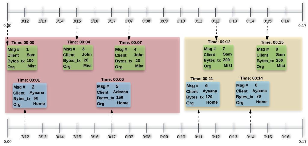
Figure 1. Kafka Messages with timeline
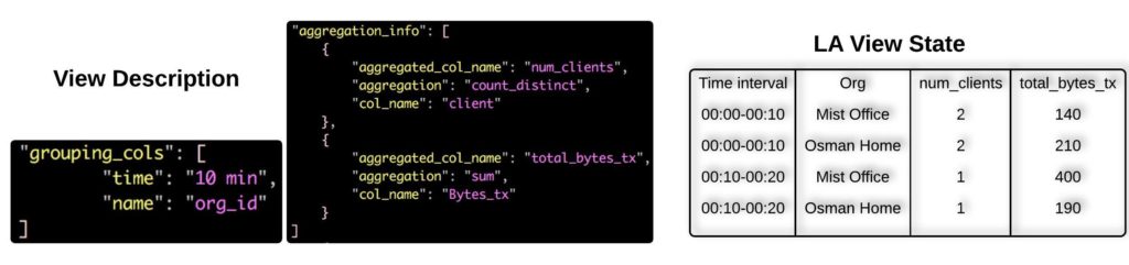
Figure 2. A view config definition and its state
Figure 1 shows incoming sample messages. For the sake of clarity, we have colored them in blue and green and separated them out vertically but they are essentially coming from the same Kafka topic/stream. The dashed arrows in Figure 1 are showing the time of arrival for each message. Figure 2 (left part) shows extract from a sample view definition. Along with some other information, LA expects two key pieces of information from view writers, i.e., grouping_cols and aggregation_info:
- grouping_cols: Aggregation requires grouping messages across certain dimensions and then applying some aggregate operations on those messages. In a LA config, you can specify the message keys on which you want to group on. In our example, we are grouping on Org and time. Since LA is a time-based aggregator, it would always group data by some time interval. In the example, we choose the time interval to be 10 minutes (10m in Figure 2 left side).
- aggregation_info: After directing the incoming messages to the right group of messages based on the the grouping_cols, we apply user defined aggregate operations on each group. LA allows you to define aggregate operations by specifying the aggregation (count_distinct or sum), the col_name (or key) of the message on which the aggregate is to be applied (client and Bytes_tx) and the name in which the resulting aggregated value would be stored, i.e., aggregated_col_name (num_clients and total_bytes_tx).
Based on the messages shown in Figure 1, LA view’s state would end up as shown in Figure 2 (right side).
System Overview
Figure 3 depicts how LA interacts with other distributed systems to reliably aggregate billions of incoming messages a day. LA uses Mesos to run all the views that users register with it. LA has its own Mesos scheduler (Figure 5) that keeps the state in Zookeeper to make sure that all the views get scheduled. The scheduler runs as a Marathon application, inspects/accepts Mesos offers and distributes views across Mesos cluster. Mesos launches LATasks (Figure 6) across the Mesos cluster after downloading the code from S3. Each of the LATasks consumes messages from Kafka, does the aggregation based on the config and writes the results to Cassandra. All LATasks periodically checkpoint entire state to S3 along with the Kafka offset to be fault tolerant. The current offsets for each view are also reported to Zookeeper which are in turn consumed by the Controller to calculate lags, i.e., how far each view is from the most recent message produced in kafka. LATasks report lots of metrics to Signalfx which are used for health monitoring as well as autoscaling LA.
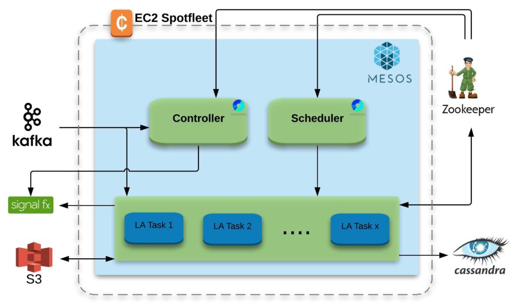
Figure 3. Live Aggregators System Overview
Embracing Unreliability to Build Highly Reliable System Using AWS Spot Instances
Netflix’s chaos monkey induces controlled faults into a system to expose unreliable software. LA’s architecture takes inducing chaos to a whole new level. LA runs entirely on AWS Spot Instances which induces uncontrolled chaos based on AWS spot market. Scheduler, controller and executors are 100% fault tolerant and can recover from day long compute outages. The fact that a fault, i.e., spot instance termination, can occur anytime and we have several of them over a single day, makes it essential for our software to be reliable from day one.
To tackle scheduler termination/restart we have designed it and kept it very simple and lightweight. It keeps minimal state and checkpoints regularly which enables our scheduler to fail and recover from the checkpointed state. Each LATask (Mesos executor) checkpoints the entire memory/state of each LA view along with the last consumed Kafka offset in S3. LA currently maintains around 750 GB of state which is checkpointed every 10 minutes on average. Figure 4 shows a spot instance termination and the corresponding view restarting with a lag of 10 minutes and recovering in the next few minutes.
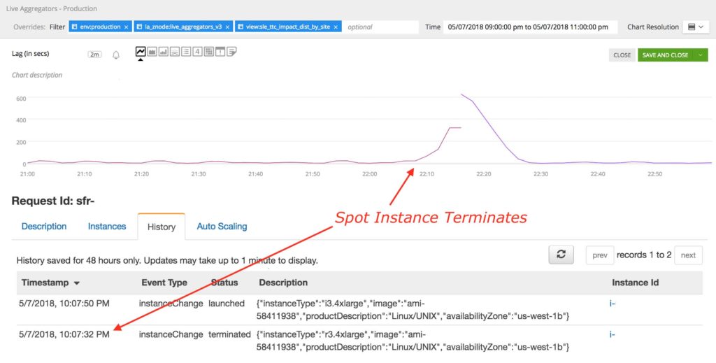
Figure 4. AWS spot instance terminates and view recovers by itself
We suffer several spot instance terminations in a day without application impact. In addition to the reliability, we are also saving ~80% in AWS compute cost by running the entire system on AWS spot instances.
How Does Scheduler Work?
An LA view could go through multiple states. Before going into scheduling details, let’s see different states a view can be in:
- Waiting: Waiting to be picked up by the scheduler. Whenever a view is deployed or encounters a failure/crash it goes into this state.
- Scheduled: Scheduler has packed the view in a LATask and asked Mesos to run it.
- Running: View is currently assigned to a healthy LATask and started its execution on Mesos.
- Disabled: As the name implies, disabled! Whenever a view fails/crashes frequently, e.g., 3 times in 10 minutes period, we mark it as Disabled. Scheduler will ignore Disabled views.
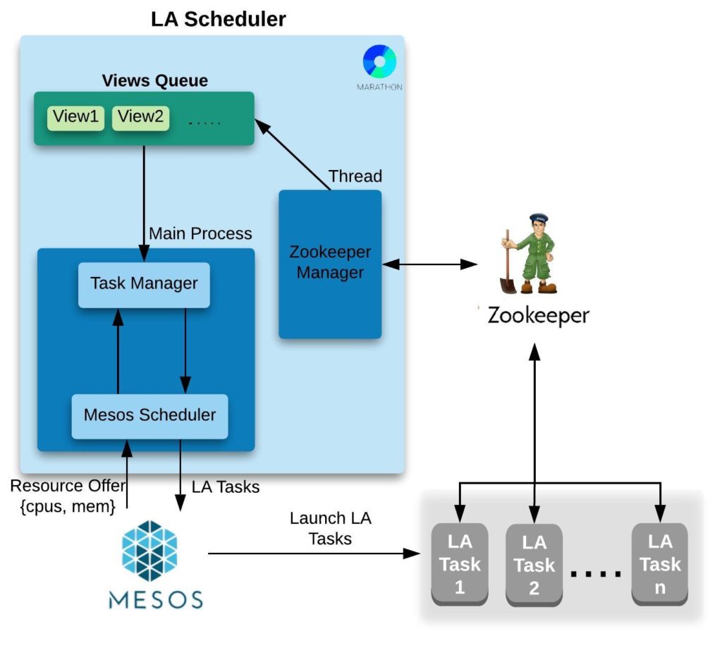
Figure 5. Live Aggregators Scheduler
There are 2 main components in Scheduler:
- Zookeeper Manager Thread: Periodically checks if a new view is deployed or if an existing view failed/crashed which needs to be rescheduled.
- Main Process: If there are views to be scheduled, the scheduler will accept Mesos resource offer and schedule those views given that the resources required by view are less than the resources offered in the current offer.
After the marathon app for the scheduler starts, the scheduler performs the following tasks:
- Creates a driver which registers LA framework with Mesos Master. Mesos then starts sending resource offers to the Mesos Scheduler.
- Instantiates Zookeeper Manager, which runs every minute, finds out if there are views in Waiting state and puts any unscheduled views in the shared Views Queue.
- When an offer is received, Mesos Scheduler checks with Task Manager if any view(s) are in Waiting state.
- Task Manager dequeues a Waiting view from the shared views queue and considers the following two possibilities:
- If mesos offer has inadequate resources, Task Manager sends a ‘resource insufficient’ message to Mesos Scheduler, or
- If mesos offer has adequate resources, Task Manager puts the view in a LATask Object and returns it to the Mesos Scheduler to launch a Mesos executor (LATask).
- Mesos Scheduler will schedule the LATask on Mesos Cluster which will get launched on a Mesos Agent.
- Our scheduler runs on top of a Mesos cluster which is running entirely on AWS spot instances. In case LA Scheduler crashes, it restarts and fetches the state of all the views from Zookeeper and continues running.
What’s inside LA Task/Executor?
LA Task is the heart of Live Aggregators which does the core job, aggregation, and writes aggregated data to Cassandra. A single LATask can run multiple views. Since Kafka Reader is compute intensive we decided to share Kafka Reader among views consuming from same stream. For the same reason LA scheduler intelligently packs views of different streams in separate LATasks. Kafka Reader writes data to shared memory for views to consume from.
Shared Memory Manager (SMM) is a separate process and gets messages in chunks from Kafka Reader. To keep the used memory low, SMM continuously cleans up all messages from memory/state which are consumed and processed by each LA view running on that LATask.
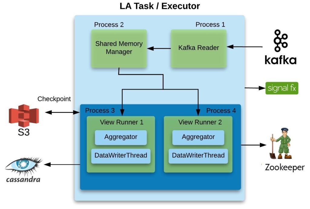
Figure 6. LATask running 2 LA views
An instance of LA View Runner takes care of one LA view and runs as a separate process. A LA View Runner has 2 main components:
-
- Aggregator: It consumes messages from SMM and does the aggregation. The type of aggregation, e.g., distinct count, sum, etc., is defined in the config as shown in Figure 2. LA supports more than 20 different aggregation types as of today. Since writing a new Aggregation type in LA is very simple, our Application Developers and Data Scientists have been adding new types increasingly. The ease of adding a new aggregation can be seen in Figure 7 for SumAggregator which does the sum aggregation in real time:
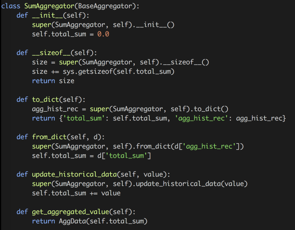
Figure 7. SumAggregator’s definition in LA
Aggregator keeps the state in memory and at a regular interval of time (defined in the view’s config) checkpoints it to S3 so that it can recover in case of crash/failure. It also writes the last processed/aggregated message offset into Zookeeper for each view. This offset is being used by Controller (explained later). LA aggregators are collectively processing billions of messages per day.
- Data Writer: It is a thread which shares the state of view with Aggregator process and writes data to Cassandra at a configurable time. Among all LA View Runners we are doing more than 200 million writes per day to Cassandra.
Each LATask emits resource utilization metrics to SignalFx for monitoring and alerting for all views. This data is being used by the Scheduler to bin pack views into LATasks in an efficient manner. We’d plan to cover it in detail in the next blog.
Controller
Controller continuously keeps track of how much work is done by LATask by checking the offset committed in ZK for that view. It also checks what is the latest offset for that view’s stream/topic in kafka, the difference of these 2 offsets is the lag for that view.
LATask also sends view’s heartbeat to Zookeeper which the Controller monitors. The controller marks a view’s state as Waiting if its heartbeat is older that a configurable threshold, e.g., 5 minutes. This typically happens when an AWS Spot instance terminates.
Monitoring and Health
We monitor our system for health and fun! We like to make sure that our infrastructure is healthy but we are also interested in learning new research-y things about our infrastructure. Most critical parts of our infrastructure are monitored and alerted using Signalfx. Let’s start with how we monitor LA’s health and then give a few examples for metrics that we use to autoscale LA.
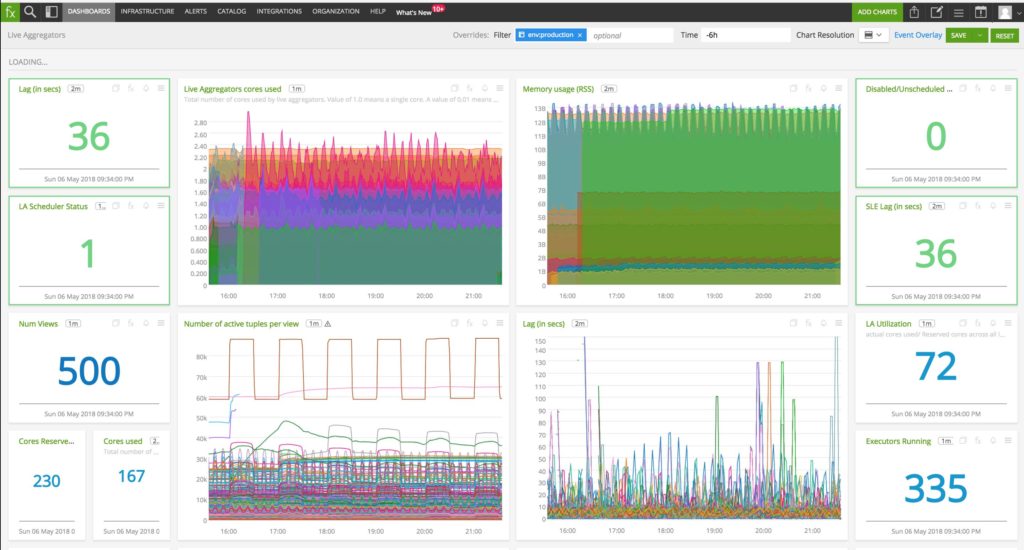
Figure 8. Critical metrics in LA
Figure 8 shows some critical metrics that are important for LA’s operation. Here’s a description for each chart:
- Lag (in secs): Tracks the amount of time each view is lagging behind real-time. The number chart shows the maximum lag for any view whereas we do keep an eye on the timeseries view to look for trends.
- Live Aggregators cores used: Displays the actual number of cores used by each LATask.
- Memory usage (RSS): The RSS memory footprint for each LATask.
- Disabled/Unscheduled Views: Number of views that aren’t scheduled or running. This should be 0.
- LA Scheduler Status: A ‘1’ means that the schedule is deployed and working fine whereas a ‘0’ implies the scheduler Mesos executor isn’t running.
- SLE Lag (in secs): Lag for views related to Service Level Expectations (SLEs) which are an essential part of our end product and hence we keep a special eye on it.
- Num Views: Tracks the total number of user-defined views deployed.
- Number of active tuples per view: Total number of active tuples/states per view.
- Lag (in secs): Shows the lag (similar to 1st metric) per view.
- LA Utilization: This is percentage of cores actually in use compared to the number of cores the scheduler reserved.
- Cores Reserved: Total number of cores reserved by the scheduler for all LATasks.
- Cores Used: Total number of cores used across all LATasks.
- Executors Running: The number of LATasks (Mesos executors) running in total.
In addition to the basic metrics mentioned above, we also monitor the detailed internal metrics of each LATask and each LA View Runner shown in Figure 9.
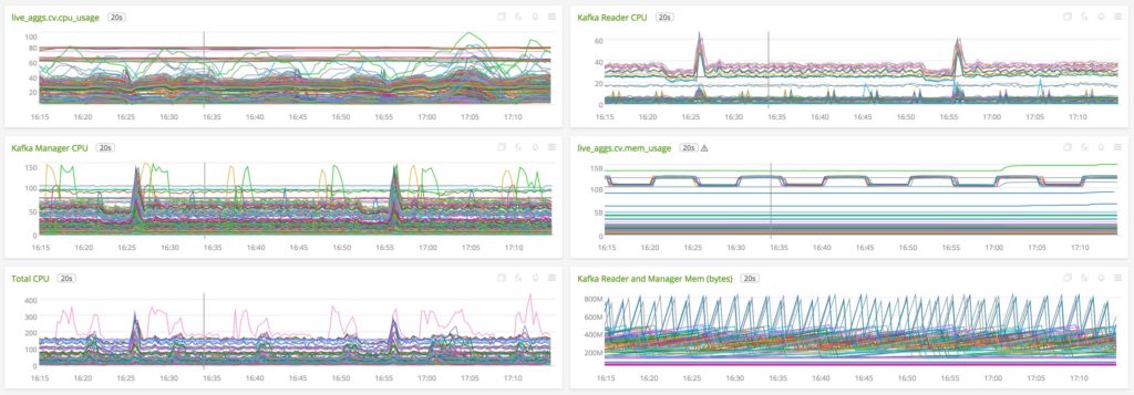
Figure 9. Detailed metrics of LA Internals
- View CPU Usage: Number of cores used by each LA View Runner process.
- Kafka Reader CPU: Number of cores used by Kafka Reader process for each LATask.
- Kafka Manager CPU: Shows the number of cores used by the python shared memory process, Shared Memory Manager, for each LATask.
- View Memory Usage: The RSS memory footprint for each LA View Runner process.
- Total CPU: The total number of cores used (not reserved) for each LATask.
- Kafka Reader and Manager Memory: RSS memory footprint for Kafka Reader and Shared Memory Manager process.
What’s next?
As Mist is growing at an accelerated rate, our load increases week over week. In addition to that our load has seasonality in it since it changes over the course of a day and also varies between different days of a week. In the next blog we plan to talk about how we are autoscaling LA to (a) keep up with the changing load; (b) ensure CPU utilization of 80% or more to deal with the trend and seasonality of our load along with saving money.
We plan to use our rich set of metrics to schedule views in an effective manner. For example, we are planning to incorporate the difference in consuming Kafka stream on different AWS instance types/sizes. Figure 10 highlights the CPU requirements (cores used) for reading the exact same Kafka stream on different instance types/sizes. This data comes directly from our production Mesos cluster where we are tracking differences in performance based on instance types/sizes. Stay tuned to hear more about how we unravel this difference in our upcoming autoscaling blog.
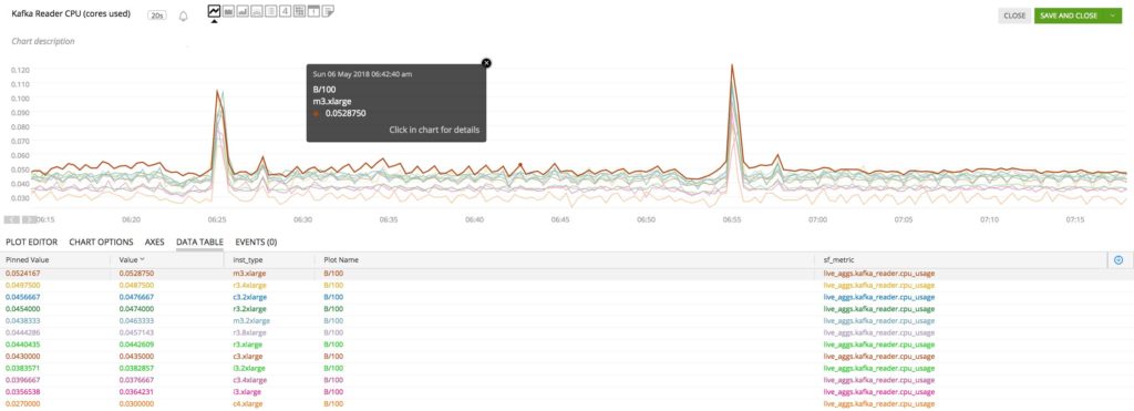
Figure 10. Kafka Reader CPU utilization for same stream on different AWS instance types/sizes
Acknowledgements
We would like to thank the following for their contributions in LA: Amarinder Singh Bindra, Jitendra Harlalka, Ebrahim Safavi and Robert Crowe.
Did This Blog Excite You?
We’re hiring rockstar distributed systems engineers to build and improve systems like Live Aggregators. Get in touch with Mist on our LinkedIn page if interested.